[EN] - excel dynamic pivot table

There is a frequent problem with frequent data analysis. And anyone that as tried this has run into this problem.
Regularly, the structure of the data is persistent (you have X number of columns, with the same type of data) but the amount is not (you can have Y rows one day/week/month and Y+1, Y-1, Y+Z..).
So when you use one of the greatest excel tools (now also available on google docs), the pivot table, every time the amount of data changes, you have to redefine the data source.

this isn't very time consuming, but it surely is ANNOYING!!! So how to automate this? Well with the named range feature (example here http://pinelasgarden.blogspot.com/2011/05/en-excel-dynamic-chart-range-with-named.html) you can have a dynamic pivot table. After adding more rows, all you need is to refresh the data source. That's all.

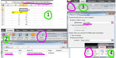
In the following image the needed steps are shown.

1 -define your data

- create a string with the data range

2- define a named range (pvt_range in the example) to hold the range's reference

3- create a pivot table

- insert the named range's name in the table/range box.

4 - after adding new rows the named range updates, and you just have to refresh the pivot table's data source.

The use of a cell for the named range isn't necessary. But for testing and changing purposes it is the best way.

For more serious implementations, the formula should be in the named range definition.